Tutorial

compas_assembly contains data structures and algorithms for modelling the individual elements of Discrete Element Assemblies or Models, and the connections and relationships between them. The package itself DOES NOT provide tools or solvers for computing contact forces between the elements, nor for analysing the stability of entire assemblies. To enable such calculations, you have to install additional solver packages such as compas_rbe.

Constructing an Assembly

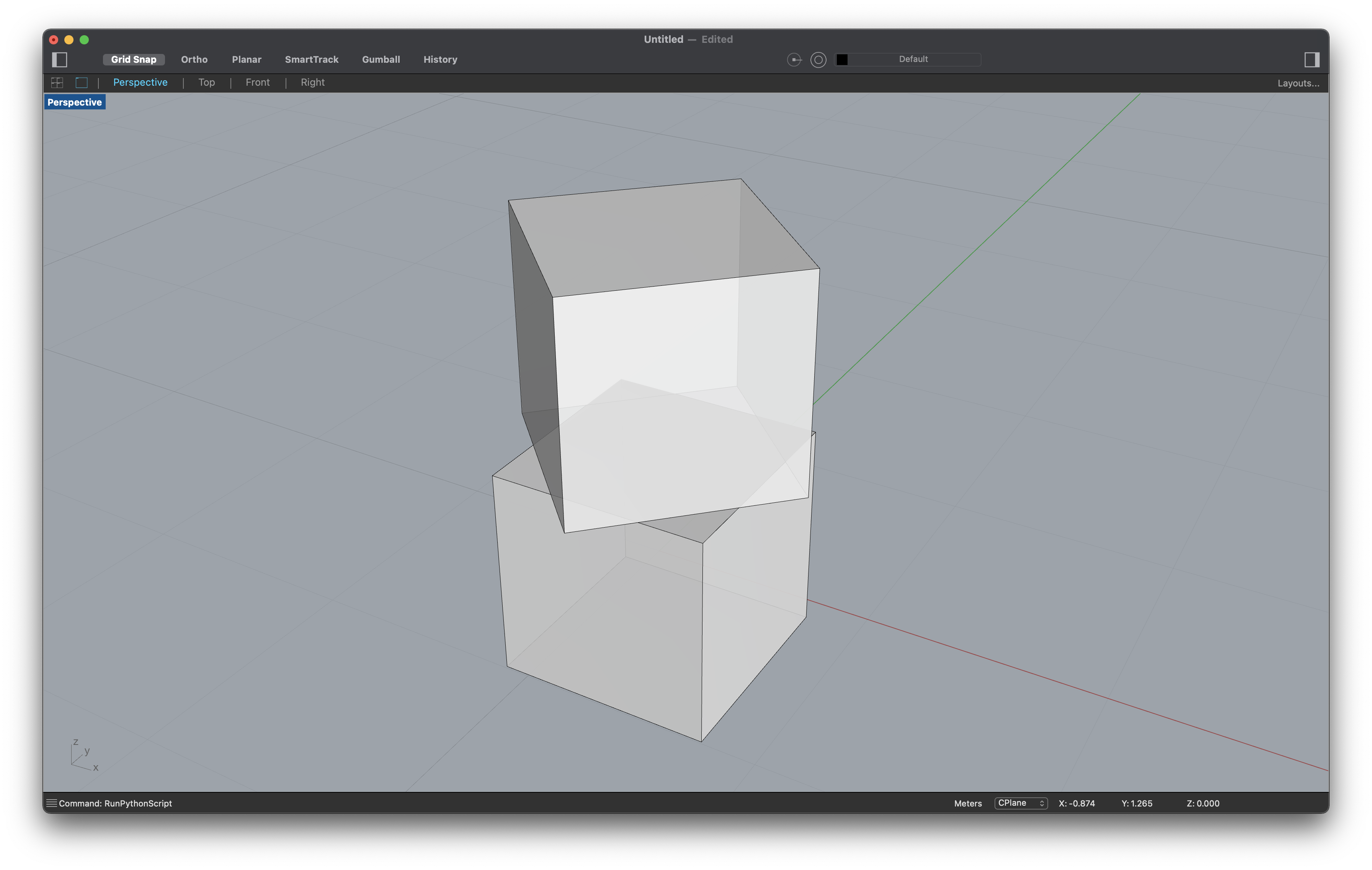
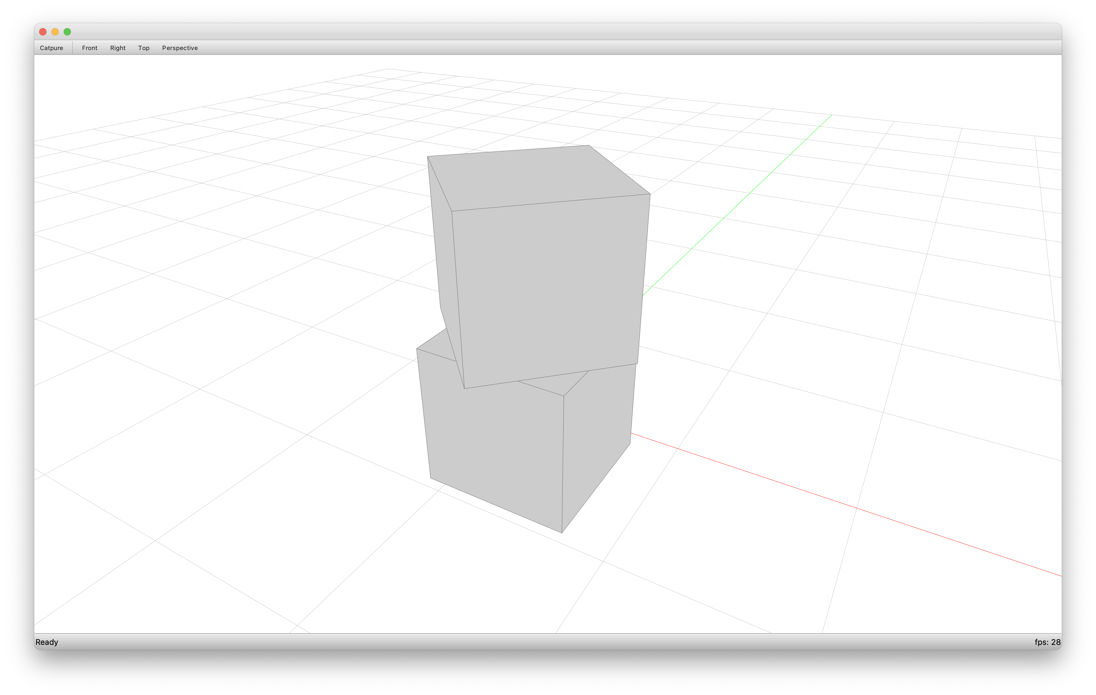
The most straightforward usage of compas_assembly is to create an empty assembly and add blocks. For example, here we create an assembly of two blocks stacked on top of each other.

from math import radians
from compas.geometry import Box, Translation, Rotation
from compas_assembly.datastructures import Block, Assembly

b1 = Block.from_shape(Box.from_width_height_depth(1, 1, 1))

T = Translation.from_vector([0, 0, 1])
R = Rotation.from_axis_and_angle([0, 0, 1], radians(45))

b2 = b1.transformed(T * R)

assembly = Assembly()

assembly.add_block(b1)
assembly.add_block(b2)

Visualization

The assembly can be visualized in Rhino/GH or Blender using artists.

Rhino

from compas_assembly.rhino import AssemblyArtist

# ...

artist = AssemblyArtist(assembly, layer='Assembly')
artist.clear_layer()

artist.draw_blocks(show_faces=True)

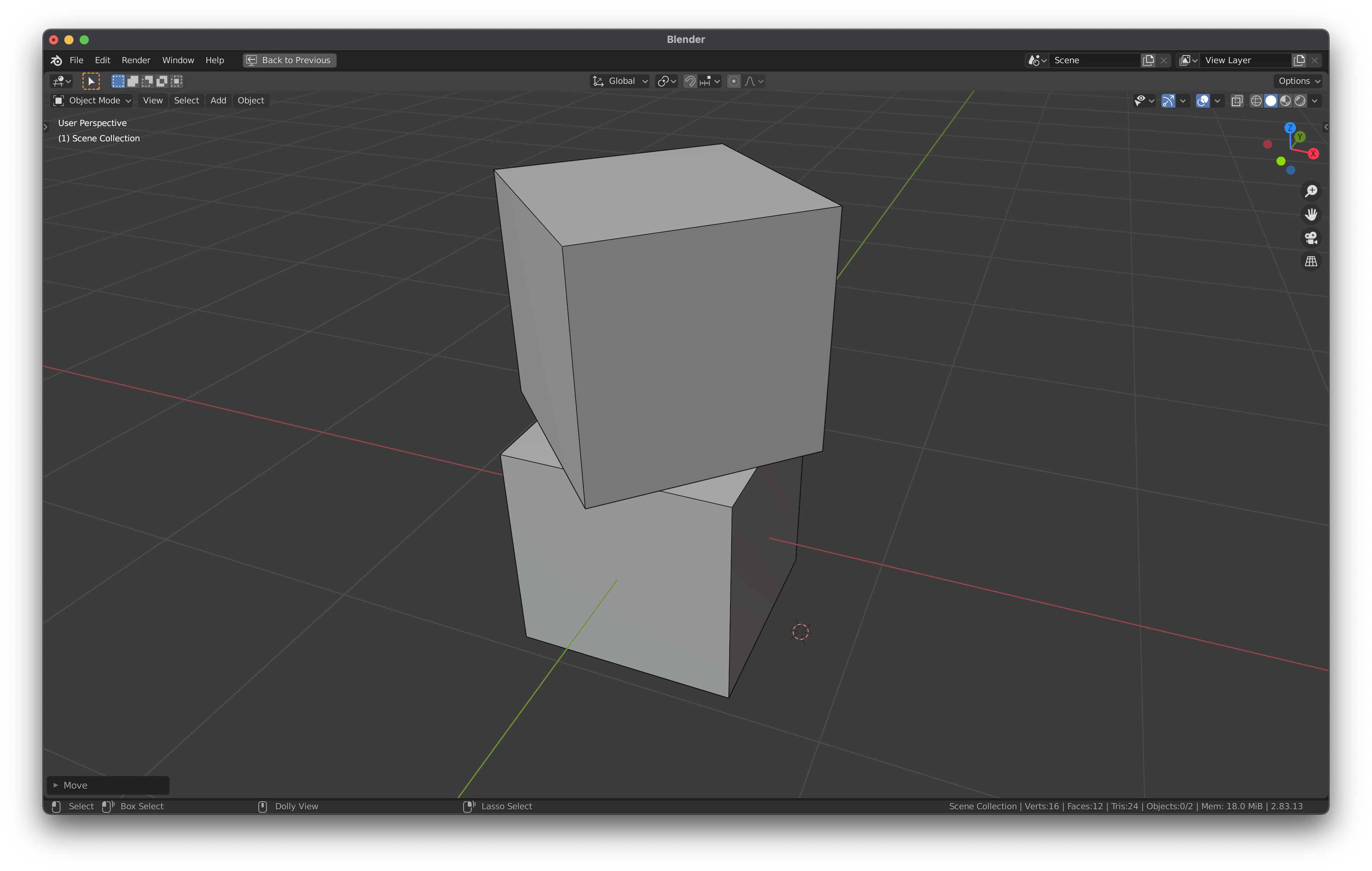
Blender

import compas_blender
from compas_assembly.blender import AssemblyArtist

# ...

compas_blender.clear()

artist = AssemblyArtist(assembly)
artist.draw_blocks()

Interfaces

At the moment, our 2-block assembly above is still simply a collection of blocks. Connections between the blocks have not been established, yet. Therefore, the graph representation of the assembly has only nodes (one per block), and no edges. The interfaces can be defined manually, if the connections and their properties are know, or using interface detection with assembly_identify_interfaces_numpy().

from compas_assembly.datastructures import assembly_interfaces_numpy

# ...

assembly_interfaces_numpy(assembly)

The interface identification algorithm uses numpy in the background (hence the suffix _numpy). In CPython environments (e.g. Blender) the function can be used directly. In Rhino, however, numpy based algorithms have to be used through a RPC proxy of compas.rpc. For more information, see the main COMPAS docs.

from compas.rpc import Proxy

proxy = Proxy('compas_assembly.datastructures')

# ...

# proxy objects can't (yet) update objects in-place
# they always return the result
assembly = proxy.assembly_interfaces(assembly)

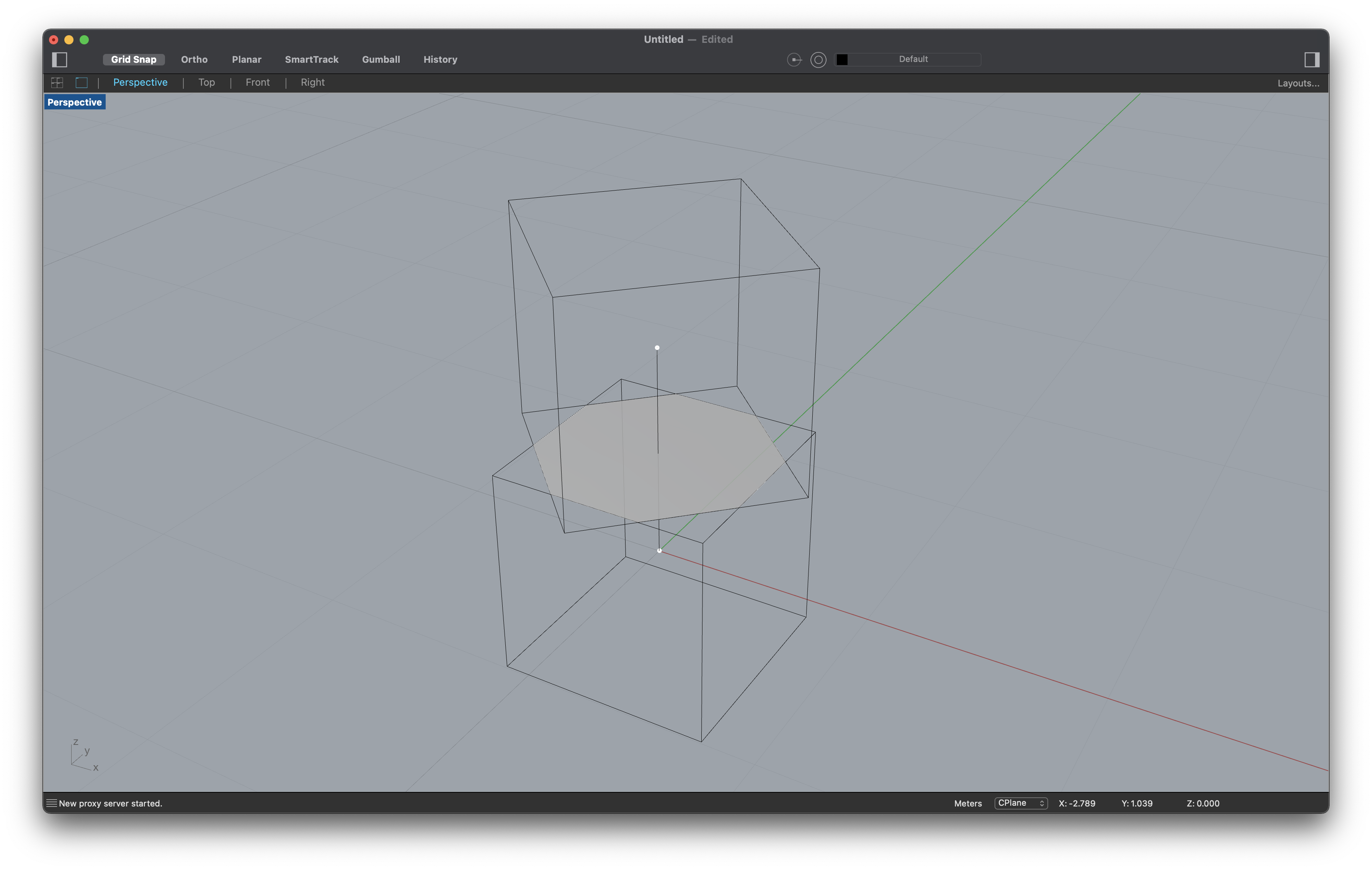
In both cases, the connections between the blocks are now encoded on the edges of the assembly network, and can be visualised.

# in Rhino

artist = AssemblyArtist(assembly)

artist.draw_nodes()
artist.draw_blocks(show_faces=False)
artist.draw_edges()
artist.draw_interfaces()

Accessing the Data

In the assembly data structure, blocks are stored as attributes of the nodes of the underlying graph or network. Each block is itself a customised mesh data structure and can be used as such to sore and retrieve data about individual elements.

assembly.number_of_nodes()  # -> the number of blocks

for node in assembly.nodes():
    block = assembly.node_attribute(node, 'block')

    centroid = block.centroid()

    for face in block.faces():
        point = block.face_centroid(face)
        normal = block.face_normal(face)

The connections between the blocks are represented by the edges of the network, and the properties of the interfaces between them are stored as interface objects in the corresponding edge data attributes.

assembly.number_of_edges()  # -> number of connections/interfaces

for edge in assembly.edges():
    interface = assembly.edge_attribute(edge, 'interface')

    interface.points
    interface.type
    interface.size
    interface.frame
    interface.forces  # -> this is empty as long as equilibrium calculations have not been performed

Serialization

Both the assembly and the individual blocks implement the COMPAS data framework. This means that entire assemblies can be saved to or loaded from a JSON file, and can be used in combination with Remote Procedure Calls from compas.rpc as we have seen earlier.

# script A

assembly.to_json('assembly.json')

# script B

assembly = Assembly.from_json('assembly.json')

Assemblies can also be stored as part of larger session files, for example to store the state of various analyses.

# script A

session = {
    'assembly': assembly,
    'solver': 'CRA',
    'solver.settings': {...},
    ...
}

compas.json_dump(session, 'session.json')

# script B

session = compas.json_load('session.json')

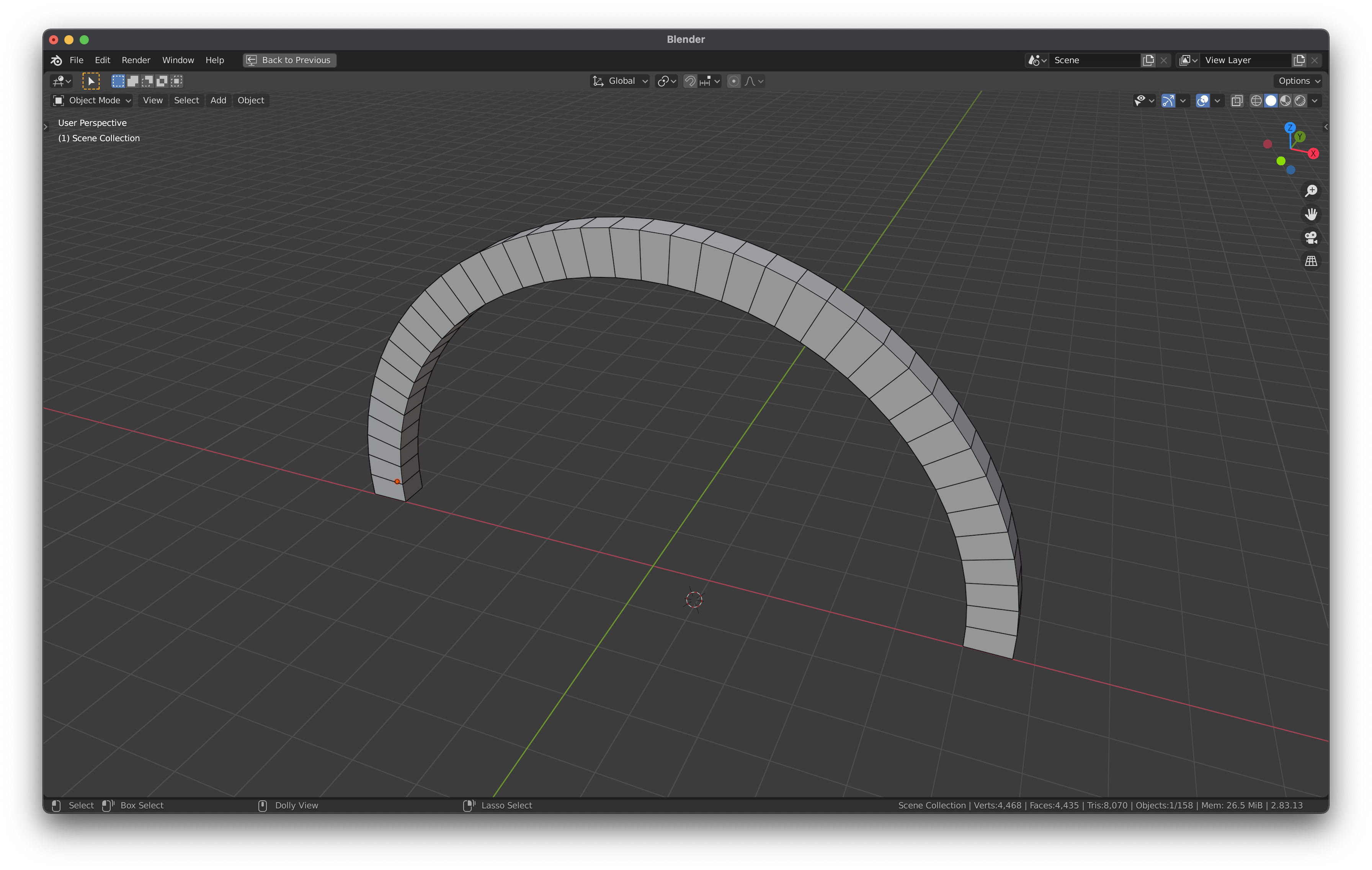
Assembly Template Geometries

In a research context, it is often useful to be able to generate variations of assemblies of well-known structural typologies, for example to generate sample data during the development of a new algorithm. For this, compas_assembly includes a growing library of geometry geometries.

arch = Arch(rise=5, span=10, thickness=0.7, depth=0.5, n=40)
assembly = Assembly.from_geometry(arch)

COMPAS Viewer

The COMPAS viewer doesn’t provide direct support for assemblies yet, but they can be visualized using a combination of a NetworkObject and multiple MeshObjects.

from compas_view2.objects import Object, NetworkObject, MeshObject
from compas_view2.app import App

Object.register(Block, MeshObject)
Object.register(Assembly, NetworkObject)

# ...

viewer = App()
viewer.add(assembly)
for node in assembly.nodes():
    block = assembly.node_attribute(node, 'block')
    viewer.add(block)
viewer.show()

Next Steps

Check out the Examples section of the docs for examples of more elaborate assemblies. Or have a look at the openMasonry project and some of the equilibrium solvers compatible with compas_assembly.