FormDiagram
This tutorial provides a quick tour of the generation of FormDiagram.
The FormDiagram can be created through a series of methods, such as:
from_library: which creates a series of parametric form diagrams that fit common rectangular and circular footprints.from_lines: create the form diagram from lines provided by the user.from_mesh: create the form diagram from meshes provided by the user, enabling the combination with different meshing strategies, or to draw the diagram freely.
The TNO library of diagrams is based on commom layouts which will be described herein.
Diagrams Library
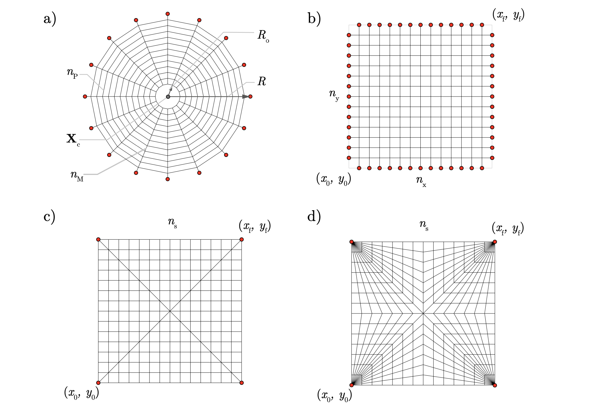
The figure above lists four parametric diagrams that can be created with TNO based on parameters.
radial diagram: polar diagram defined by two discretisation parameters being the number of meridians
 and the number of circular parallels, or hoops
  . The location is defined by the central point position
  and the size by the radius
  . Oculus openings can be considered with the parameter
  . This diagram can be used to analyse problems on domes. The code to generate this diagram considering
 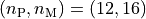 ,
,  ,
,  and
and  diagram can be written in two forms:
Long form:
from compas_tno.diagrams import FormDiagram
data = {
    'type': 'radial_fd',
    'center': [5.0, 5.0],
    'radius': 5.0,
    'discretisation': [12, 16],
    'r_oculus': 0.75
}
form = FormDiagram.from_library(data)
Simple form:
from compas_tno.diagrams import FormDiagram
form = FormDiagram.create_circular_radial_form(center=[5.0, 5.0],
                                               radius=5.0,
                                               discretisation=[12, 16],
                                               r_oculus=0.75)
orthogonal diagram: the orthogonal diagram is defined through two discretisation parameters (
 ), and the start and end dimensions of two opposite corners
 ![[[x_\mathrm{0}, x_\mathrm{f}], [y_\mathrm{0}, y_\mathrm{f}]]](../_images/math/308c39dabf903286a4d04ee8f3987c6cc0a50682.png) . This diagram is suitable for performing analysis of continuously supported vaults, such as pavillion vaults. The square orthogonal diagram is presented in the Figure above can be generated by the following code:
. This diagram is suitable for performing analysis of continuously supported vaults, such as pavillion vaults. The square orthogonal diagram is presented in the Figure above can be generated by the following code:
from compas_tno.diagrams import FormDiagram
form = FormDiagram.create_ortho_form(xy_span=[[0.0, 10.0], [0.0, 10.0]],
                                     discretisation=[14, 14],
                                     fix='all')
cross diagram: the cross diagram corresponds to the orthogonal diagram added with the main diagonals, defined through identical parameters as in the orthogonal case. This diagram is used in the cross vault example. The cross diagram with
 can be constructed with:
from compas_tno.diagrams import FormDiagram
form = FormDiagram.create_cross_form(xy_span=[[0.0, 10.0], [0.0, 10.0]],
                                     discretisation=14)
fan diagram: unlike the orthogonal arrangement, the parallel segments arriving at the diagonals are directed to the corners. The parameters are identical to the ones necessary to construct the cross diagram. This diagram is used in the alternative cross vault example. The cross diagram with
can be constructed with:
from compas_tno.diagrams import FormDiagram
form = FormDiagram.create_fan_form(xy_span=[[0.0, 10.0], [0.0, 10.0]],
                                   discretisation=14)
To further explore the library of parametric diagrams, check the FormDiagram full documentation.
Modifying diagrams
Pragmatic geometric modifications can also be applied to patterns in TNO, increasing the diversity of patterns used to study masonry problems. Some of these transformations are presented illustrated below:
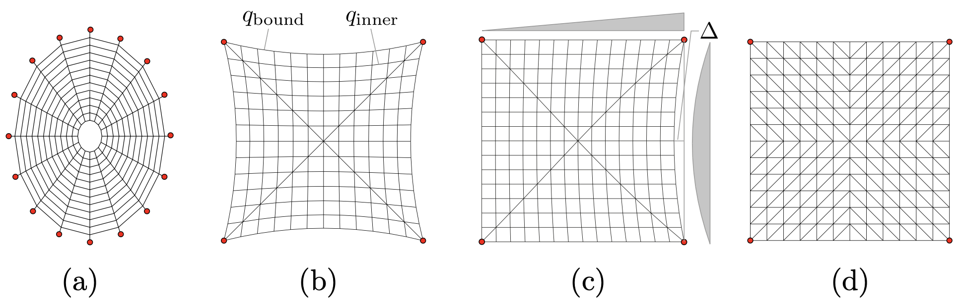
scale and shear: scaling and shear can be applied from the COMPAS framework, see
compas.geometry.Scaleandcompas.geometry.Shear.sag: curving the unsupported bounds inwards can be done by applying sag to the pattern using the method
slide_pattern_inwards.slide: sliding the nodes horizontally is necessary for applying horizontal forces in patterns with unsupported boundaries, a helper method
slide_diagramhas been added to ease this process.adding members: members can be added using helper functions such as adding lines to supports with method
form_add_lines_support.
TNO Plotter
For 2D visualisation, the TNO Plotter can be used. This matplotlib based visualisation enable to draw the form diagrams and configure their thickness, color, etc. To visualise the cross form diagram from this example, the code is:
from compas_tno.diagrams import FormDiagram
from compas_tno.plotters import TNOPlotter
form = FormDiagram.create_cross_form(xy_span=[[0.0, 10.0], [0.0, 10.0]], discretisation=14)
plot = Plotter(form)
plot.draw_form()
plot.draw_supports()
plot.show()